Spatial partitioning in Dask-GeoPandas

Dask-GeoPandas has implemented spatial_shuffle method to repartition Dask.GeoDataFrames geographically. For those who are not familiar with Dask, a Dask DataFrame is internally split into many partitions, where each partition is a Pandas DataFrame. Partitions are split vertically along the index;

There are numerous strategies that can be used to partition Dask DataFrames, which determine how the elements of a DataFrame are separated into each resulting partition. Common strategies to partition Dask DataFrames include using a fixed number of partitions or partitions based on column values. Dask-GeoPandas can partition GeoDataFrames by taking advantage of their spatial structure.

In the rest of this notebook, we use an example dataset to describe how Dask-GeoPandas takes advantage of this spatial structure and some best practices.

import geopandas
import dask_geopandas
import matplotlib.pyplot as plt

/Users/tstatham/anaconda3/envs/gsoc/lib/python3.9/site-packages/geopandas/_compat.py:111: UserWarning: The Shapely GEOS version (3.8.0-CAPI-1.13.1 ) is incompatible with the GEOS version PyGEOS was compiled with (3.9.1-CAPI-1.14.2). Conversions between both will be slow.
  warnings.warn(

We first begin by reading USA boundaries from gadm.org

path = "https://geodata.ucdavis.edu/gadm/gadm4.0/gpkg/gadm40_USA.gpkg"

usa = geopandas.read_file(path, layer="ADM_1")
usa.head()

	ID_0	COUNTRY	ID_1	NAME_1	VARNAME_1	NL_NAME_1	TYPE_1	ENGTYPE_1	CC_1	HASC_1	ISO_1	geometry
0	USA	United States	USA.1_1	Alabama	AL|Ala.		State	State		US.AL		MULTIPOLYGON (((-88.12063 30.23321, -88.12122 ...
1	USA	United States	USA.2_1	Alaska	AK|Alaska		State	State		US.AK		MULTIPOLYGON (((179.20071 51.35992, 179.20010 ...
2	USA	United States	USA.3_1	Arizona	AZ|Ariz.		State	State		US.AZ		MULTIPOLYGON (((-110.87869 31.33084, -110.9720...
3	USA	United States	USA.4_1	Arkansas	AR|Ark.		State	State		US.AR		MULTIPOLYGON (((-91.90713 33.00801, -92.01710 ...
4	USA	United States	USA.5_1	California	CA|Calif.		State	State		US.CA		MULTIPOLYGON (((-117.23300 32.77416, -117.2330...

# Filter and rename cols
usa = usa[["NAME_1", "geometry"]].rename(columns={"NAME_1": "State"})
usa.info()

<class 'geopandas.geodataframe.GeoDataFrame'>
RangeIndex: 51 entries, 0 to 50
Data columns (total 2 columns):
 #   Column    Non-Null Count  Dtype   
---  ------    --------------  -----   
 0   State     51 non-null     object  
 1   geometry  51 non-null     geometry
dtypes: geometry(1), object(1)
memory usage: 944.0+ bytes

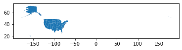
usa.plot()

<AxesSubplot:>

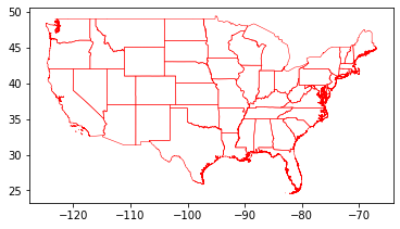
We can quickly filter for Contiguous United States, which represents the 48 joining states and the District of Columbia (DC) by the cx method. This filters out any geometries using a bounding box.

us_cont = usa.cx[-150:-50, 20:50]
us_cont.info()

<class 'geopandas.geodataframe.GeoDataFrame'>
Int64Index: 49 entries, 0 to 50
Data columns (total 2 columns):
 #   Column    Non-Null Count  Dtype   
---  ------    --------------  -----   
 0   State     49 non-null     object  
 1   geometry  49 non-null     geometry
dtypes: geometry(1), object(1)
memory usage: 1.1+ KB

us_cont.plot(facecolor="none", linewidth=0.5, edgecolor="red")

<AxesSubplot:>

We can then transform the geopandas.GeoDataFrame to a dask_geopandas.GeoDataFrame, with a fixed number of arbitrary partitions - this does not yet spatially partition a Dask GeoDataFrame.

Note

We can also read (and export) parquet files in Dask-GeoPandas containing spatially partitioned data.

d_gdf = dask_geopandas.from_geopandas(us_cont, npartitions=4)
d_gdf

Dask-GeoPandas GeoDataFrame Structure:

	State	geometry
npartitions=4
0	object	geometry
15	...	...
28	...	...
41	...	...
50	...	...

Dask Name: from_pandas, 4 tasks

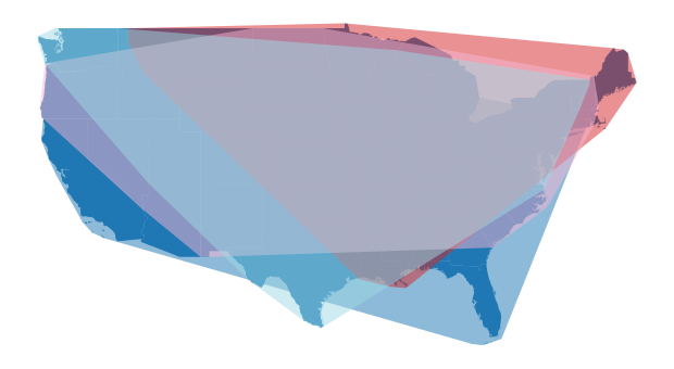
By visualising the convex hull of each partition, we can get a feel for how the Dask-GeoDataFrame has been partitioned using the fixed number. A useful spatial partitioning scheme is one that minimises the degree of spatial overlap between partitions. By default, the fixed number of partitions does a poor job of spatially partitioning our example data - there is a high degree of overlap between partitions.

d_gdf.calculate_spatial_partitions() # convex hull
d_gdf.spatial_partitions

0    POLYGON ((-81.96430 24.52042, -82.87569 24.610...
1    POLYGON ((-89.42000 28.92833, -90.92028 29.048...
2    POLYGON ((-109.04997 31.33190, -114.63287 35.0...
3    POLYGON ((-97.40186 25.83808, -97.40523 25.838...
dtype: geometry

fig, ax = plt.subplots(1,1, figsize=(12,6))
us_cont.plot(ax=ax)
d_gdf.spatial_partitions.plot(ax=ax, cmap="tab20", alpha=0.5)
ax.set_axis_off()
plt.show()

Spatial partitioning a Dask GeoDataFrames is done using spatial_shuffle, which is based on Dasks set_index and spatial sorting.

Spatial sorting methods

spatial_shuffle supports three different partitioning methods, which provide a simple and relatively inexpensive way of representing two-dimensional objects in one-dimensional space. These are called using the by parameter;

1. Hilbert distance (default)

2. Morton distance

3. Geohash

The first two methods are space-filling curves, which are lines that pass through every point in space, in a particular order and pass through points once only, so that each point lies a unique distance along the curve. The range of both curves contain the entire 2-dimensional unit square, which means that the Hilbert and Morton curves can handle projected coordinates. In general, we recommend the default Hilbert distance because it has better order-preserving behaviour. This is because the curve holds a remarkable mathematical property, where the distance between two consecutive points along the curve is always equal to one. By contrast, the Morton distance or “Z-order curve” does not hold this property and there are larger “jumps” in distances between two consecutive points. Currently, calculated distances along the curves are based on the mid points of geometries. Whilst this is inexpensive, mid points do not represent complex geometries well. Future work will examine various methods for better representing complex geometries.

The Geohash, not to be confused with geohashing, is a hierarchical spatial data structure, which subdivides space into buckets of grid shape. Whilst the Geohash does allow binary searchers or spatial indexing, like rtree or quadtree, Geohash is limited to encoding latitude and longitude coordinates. The Geohash can be represented either as text string or integers, where the longer the string/integer is, the more precise the grid shape will be.

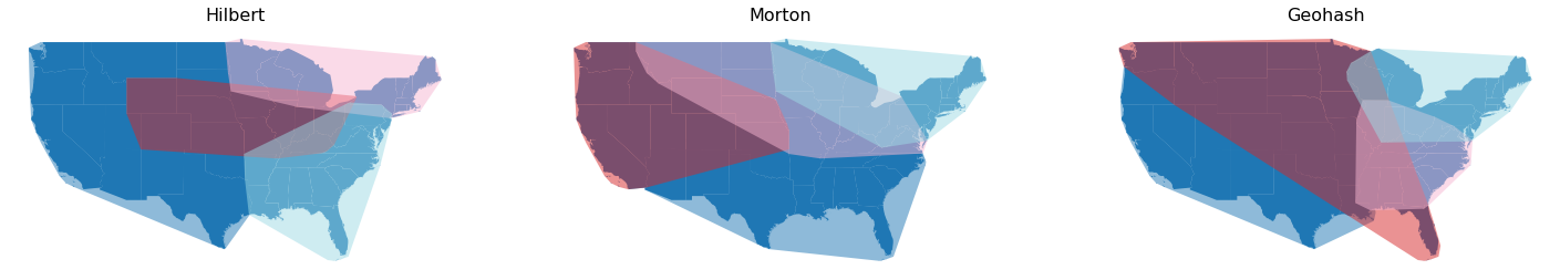
Below we compare the different sorting methods using the default parameters. All 3 sorting methods reduce the degree of spatial overlap but this still remains high and could be further improved by controlling specific parameters.

hilbert = d_gdf.spatial_shuffle(by="hilbert")
morton = d_gdf.spatial_shuffle(by="morton")
geohash = d_gdf.spatial_shuffle(by="geohash")

fig, axes = plt.subplots(nrows=1,ncols=3, figsize=(25,12))
ax1, ax2, ax3 = axes.flatten()

for ax in axes:
    us_cont.plot(ax=ax)

hilbert.spatial_partitions.plot(ax=ax1, cmap="tab20", alpha=0.5)
morton.spatial_partitions.plot(ax=ax2, cmap="tab20", alpha=0.5)
geohash.spatial_partitions.plot(ax=ax3, cmap="tab20", alpha=0.5)

[axi.set_axis_off() for axi in axes.ravel()]

ax1.set_title("Hilbert", size=16)
ax2.set_title("Morton", size=16)
ax3.set_title("Geohash", size=16)

plt.show()

Number of partitions

The first parameter is the npartitions or number of partitions. The default npartitions is the same number of partitions as the original Dask GeoDataFrame. Increasing the number of partitions will reduce the degree of spatial overlap between partitions.

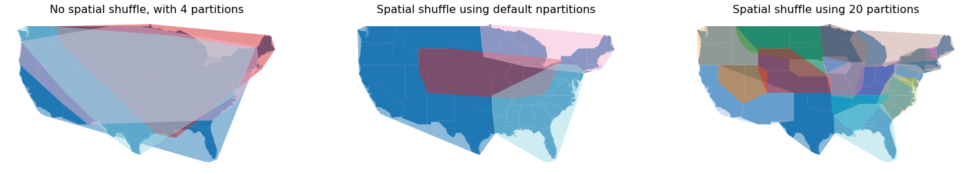
Below shows a comparison between the different approaches;

1. The original Dask GeoDataFrame with no spatial partitioning

2. The same Dask GeoDataFrame spatially shuffled with the default number of partitions as the original Dask GeoDataFrame

3. The same Dask GeoDataFrame using 20 partitions.

It’s quite clear that using 20 partitions does reduce the overall degree of spatial overlap between partitions. The number of partitions depends on your data structure and how you plan to use your data.

hilbert20 = d_gdf.spatial_shuffle(by="hilbert", npartitions=20)

fig, axes = plt.subplots(nrows=1,ncols=3, figsize=(25,12))
ax1, ax2, ax3 = axes.flatten()

for ax in axes:
    us_cont.plot(ax=ax)

d_gdf.spatial_partitions.plot(ax=ax1, cmap="tab20", alpha=0.5)
hilbert.spatial_partitions.plot(ax=ax2, cmap="tab20", alpha=0.5)
hilbert20.spatial_partitions.plot(ax=ax3, cmap="tab20", alpha=0.5)

[axi.set_axis_off() for axi in axes.ravel()]

ax1.set_title("No spatial shuffle, with 4 partitions", size=16)
ax2.set_title("Spatial shuffle using default npartitions", size=16)
ax3.set_title("Spatial shuffle using 20 partitions", size=16)

plt.show()

Level of precision

The level parameter represents the precision of each partitioning method. This defaults to 16 for both the Hilbert and Morton distance. However, the Geohash method does not use this parameter and defaults to the integer representation. We have found there are no significant penalties in selecting the maximum precision.

Summary

Dask offers some guidance on partitioning Pandas DataFrames, which also applies to Dask-GeoPandas GeoDataFrames;

1. Try GeoPandas first - GeoPandas can often be faster and easier to use than Dask-GeoPandas for small data problems.

2. If you are running into memory and/or performance issues with GeoPandas, then the number of partitions of a Dask-GeoDataFrame should fit comfortably into memory, each smaller than a gigabyte in size. So if you are handling a 10GB dataset, first try using 10 partitions.

3. One common use case of Dask-GeoPandas is to read in large amounts of data, reduce it down and then iterate on a much smaller amount of data. This may only be for a single component of your workflow, so it might make sense to revert back to GeoPandas once this component is complete.